Unsupervised Anomaly Detection with One-Class SVM

How to identify anomalies with One-Class SVM.

Introduction

Anomaly detection (outlier detection, novelty detection) is the identification of rare observations that differ substantially from the vast majority of the data \(^4\).

I would like to point out an important distinction \(^3\):

• Outlier detection: The training data contains outliers. Estimators try to fit the regions where the training data is the most concentrated.
• Novelty detection: The training data does not contain outliers. Estimators try to detect whether a new observation is an outlier.

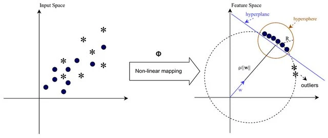
In short, SVMs separates two classes using a hyperplane with the largest possible margin. On other side, One-Class SVMs try to identify smallest hypersphere which contains most of the data points\(^4\).

Source: \(^5\)

Example

Dataset was downloaded from ODDS \(^{1,2}\). The original dataset contains labels but we’ll not use them.

data = arff.loadarff('seismic-bumps.arff')
df = pd.DataFrame(data[0])

for col in df:
    if isinstance(df[col][0], bytes):
        df[col] = df[col].str.decode("utf8")

Markdown(tabulate(
  df.head(), 
  headers=df.columns
))

	seismic	seismoacoustic	shift	genergy	gpuls	gdenergy	gdpuls	ghazard	nbumps	nbumps2	nbumps3	nbumps4	nbumps5	nbumps6	nbumps7	nbumps89	energy	maxenergy	class
0	a	a	N	15180	48	-72	-72	a	0	0	0	0	0	0	0	0	0	0	0
1	a	a	N	14720	33	-70	-79	a	1	0	1	0	0	0	0	0	2000	2000	0
2	a	a	N	8050	30	-81	-78	a	0	0	0	0	0	0	0	0	0	0	0
3	a	a	N	28820	171	-23	40	a	1	0	1	0	0	0	0	0	3000	3000	0
4	a	a	N	12640	57	-63	-52	a	0	0	0	0	0	0	0	0	0	0	0

Let’s drop categorical columns and class column:

df = df.loc[:, ~df.columns.isin(['seismic', 'seismoacoustic', 'shift', 'ghazard', 'class'])]

Markdown(tabulate(
  df.head(), 
  headers=df.columns
))

	genergy	gpuls	gdenergy	gdpuls	nbumps	nbumps2	nbumps3	nbumps4	nbumps5	nbumps6	nbumps7	nbumps89	energy	maxenergy
0	15180	48	-72	-72	0	0	0	0	0	0	0	0	0	0
1	14720	33	-70	-79	1	0	1	0	0	0	0	0	2000	2000
2	8050	30	-81	-78	0	0	0	0	0	0	0	0	0	0
3	28820	171	-23	40	1	0	1	0	0	0	0	0	3000	3000
4	12640	57	-63	-52	0	0	0	0	0	0	0	0	0	0

Split data to train and test sets:

X_train, X_test = train_test_split(df, test_size = 0.2)

SVM tries to maximize distance between the hyperplane and the support vectors. If some features have very big values, they will dominate the other features. So it is important to rescale data while using distance based methods:

scaler = MinMaxScaler()
X_train_scaled = scaler.fit_transform(X_train)
X_test_scaled = scaler.transform(X_test)

Markdown(tabulate(
  X_train_scaled[:5], 
  headers=df.columns,
))

Scaled Train set

genergy	gpuls	gdenergy	gdpuls	nbumps	nbumps2	nbumps3	nbumps4	nbumps5	nbumps6	nbumps7	nbumps89	energy	maxenergy
0.0115891	0.085282	0.0775541	0.0792291	0.111111	0	0.142857	0	0	0	0	0	0.00660066	0.00666667
0.0122517	0.146722	0.0507084	0.0770878	0.222222	0.25	0	0	0	0	0	0	0.00363036	0.00233333
0.0112539	0.10133	0.231171	0.143469	0	0	0	0	0	0	0	0	0	0
0.00888829	0.0790922	0.0581655	0.0760171	0	0	0	0	0	0	0	0	0	0
0.0148177	0.169188	0.248322	0.280514	0.111111	0	0.142857	0	0	0	0	0	0.0231023	0.0233333

Markdown(tabulate(
  X_test_scaled[:5], 
  headers=df.columns,
))

Scaled Test set

genergy	gpuls	gdenergy	gdpuls	nbumps	nbumps2	nbumps3	nbumps4	nbumps5	nbumps6	nbumps7	nbumps89	energy	maxenergy
0.0282483	0.274874	0.111111	0.205567	0.555556	0.25	0.285714	0.333333	0	0	0	0	0.09967	0.0666667
0.00104795	0.00504356	0.0790455	0.0620985	0	0	0	0	0	0	0	0	0	0
0.00152954	0.0389729	0.0260999	0.0449679	0	0	0	0	0	0	0	0	0	0
0.0598871	0.0825309	0.126771	0.187366	0	0	0	0	0	0	0	0	0	0
0.0218027	0.182714	0.189411	0.22591	0.111111	0	0.142857	0	0	0	0	0	0.00330033	0.00333333

Apply T-SNE for 2-d visualization:

t_sne = TSNE(n_components=2, 
             learning_rate = 'auto',
             init='pca',
             random_state=1234)
             
X_train_viz = t_sne.fit_transform(X_train_scaled)
X_test_viz = t_sne.fit_transform(X_test_scaled)

px.scatter(x=X_train_viz[:,0], y=X_train_viz[:,1], title="Train set")

px.scatter(x=X_test_viz[:,0], y=X_test_viz[:,1], title="Test set")

Let’s train and predict:

# We assume that the proportion of outliers in the data set is 0.15
clf = OCSVM(contamination=0.15)
clf.fit(X_train_scaled)

X_train_pred = clf.labels_  # binary labels (0: inliers, 1: outliers)
X_train_scores = clf.decision_scores_  # raw outlier scores

X_test_pred = clf.predict(X_test_scaled)  # outlier labels (0 or 1)
X_test_scores = clf.decision_function(X_test_scaled)  # outlier scores

Replace prediction classes (0 & 1) with strings:

labels = {0: 'inlier', 1: 'outlier'}

X_train_pred = np.vectorize(labels.get)(X_train_pred)
X_test_pred = np.vectorize(labels.get)(X_test_pred)

Visualize with T-SNE:

px.scatter(x=X_train_viz[:,0], y=X_train_viz[:,1], title="Train set", color=X_train_pred)

px.scatter(x=X_test_viz[:,0], y=X_test_viz[:,1], title="Test set",  color=X_test_pred)

Full source code: https://github.com/mrtkp9993/MyDsProjects/tree/main/AnomalyOcsvm

References

\(^1\) http://odds.cs.stonybrook.edu/seismic-dataset/

\(^2\) Saket Sathe and Charu C. Aggarwal. LODES: Local Density meets Spectral Outlier Detection. SIAM Conference on Data Mining, 2016.

\(^3\) https://scikit-learn.org/stable/modules/outlier_detection.html

\(^4\) Contributors to Wikimedia projects. (2022, September 03). Anomaly detection - Wikipedia. Retrieved from https://en.wikipedia.org/w/index.php?title=Anomaly_detection&oldid=1108262189

\(^5\) Yengi, Yeliz & Kavak, Adnan & Arslan, Huseyin. (2020). Physical Layer Detection of Malicious Relays in LTE-A Network Using Unsupervised Learning. IEEE Access. PP. 1-1. 10.1109/ACCESS.2020.3017045.

Citation

BibTeX citation:

@online{koptur2022,
  author = {Koptur, Murat},
  title = {Unsupervised {Anomaly} {Detection} with {One-Class} {SVM}},
  date = {2022-09-10},
  url = {https://www.muratkoptur.com/MyDsProjects/AnomalyOcsvm/Analysis.html},
  langid = {en}
}

For attribution, please cite this work as:

Koptur, Murat. 2022. “Unsupervised Anomaly Detection with One-Class SVM.” September 10, 2022. https://www.muratkoptur.com/MyDsProjects/AnomalyOcsvm/Analysis.html.