Under the hood: Expectation Maximization (EM)

How to estimate parameters if our data contains missing values or variables?

Introduction

Source: https://jonathan-hui.medium.com/machine-learning-expectation-maximization-algorithm-em-2e954cb76959

If data contains missing values or latent (unobserved) variables, we cannot use the MLE for estimating parameters since the likelihood will be based on both observed and unobserved data. Expectation-maximization (EM) algorithm was developed by Dempster, Laird and Rubin for to find a maximum likelihood estimate of parameters in presence of missing or unobserved data \(^2\).

Assume that the complete dataset consists of \(\mathcal{Z}=(\mathcal{X},\mathcal{Y})\) but that only \(\mathcal{X}\) is observed. Denote the (complete-data) log-likelihood as \(l(\theta;\mathcal{X},\mathcal{Y})\) where \(\theta\) is the unknown parameter vector which we want to estimate. Then, algorithm iteratively applies these two steps:

Expectation step (E-step): Calculate the expected value of complete-data log-likelihood function \(l(\theta;\mathcal{X},\mathcal{Y})\) given the observed data and the current parameter estimate \(\theta_{\text{old}}\):

\[ \begin{align*} Q(\theta;\theta_\text{old}) &:= \mathbb{E}[l(\theta;\mathcal{X},\mathcal{Y})|\mathcal{X},\theta_\text{old}]\\ &= \int l(\theta;\mathcal{X},y)p(y|\mathcal{X},\theta_{\text{old}})dy \end{align*} \]

where \(p(\cdot|\mathcal{X},\theta_{\text{old}})\) is the conditional density of \(\mathcal{Y}\) given observed data \(\mathcal{X}\), and assuming \(\theta=\theta_\text{old}\).

Maximization step (M-step): Maximize the expectation over \(\theta\):

\[ \theta_\text{new}:=\max_\theta Q(\theta;\theta_{\text{old}}) \]

and set \(\theta_\text{old}=\theta_\text{new}\). Repeat these two steps until the sequence of \(\theta_\text{new}\)’s converge \(^1\).

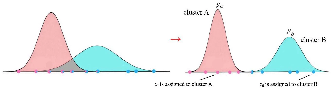
One can ask “How can we choose the initial values?”: for finite mixture distributions, we can estimate initial values for each distribution by K-means.

Example - Finite Mixture Gaussians

Let’s generate the data:

set.seed(1234)

n1 <- 100
mu1 <- 5
sigma1 <- 2

n2 <- 50
mu2 <- 7
sigma2 <- 1.5

d1 <- rnorm(n1, mu1, sigma1)
d2 <- rnorm(n2, mu2, sigma2)

d <- c(d1, d2) # combine data

Let’s look our generated data:

hist(d)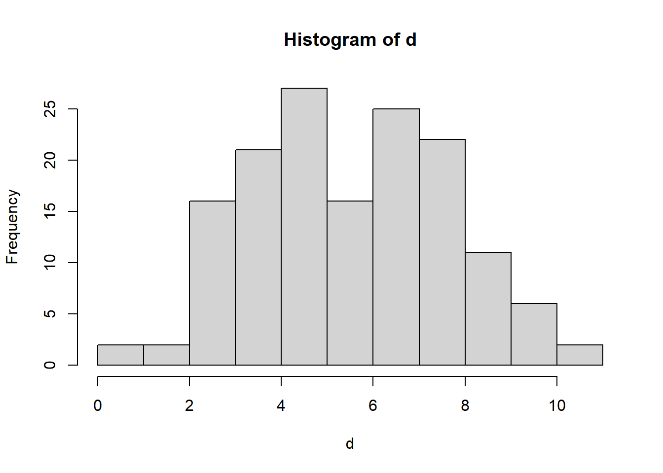

We need to estimate initial values for EM algorithm. I’ll use K-means estimates for initial values:

clusters <- kmeans(d,2)$cluster
mu1i <- mean(d[clusters==1])
mu2i <- mean(d[clusters==2])
sigma1i <- sd(d[clusters==1])
sigma2i <- sd(d[clusters==2])
pi1i <- sum(clusters==1)/length(clusters)
pi2i <- sum(clusters==2)/length(clusters)

Apply algorithm:

# Source: https://rpubs.com/H_Zhu/246450
Q <- 0
Q[2] <- sum(log(pi1i)+log(dnorm(d, mu1i, sigma1i))) + sum(log(pi2i)+log(dnorm(d, mu2i, sigma2i)))

k <- 2

while (abs(Q[k]-Q[k-1])>=1e-6) {
  # E step
  comp1 <- pi1i * dnorm(d, mu1i, sigma1i)
  comp2 <- pi2i * dnorm(d, mu2i, sigma2i)
  comp.sum <- comp1 + comp2
  
  p1 <- comp1/comp.sum
  p2 <- comp2/comp.sum
  
  # M step
  pi1i <- sum(p1) / length(d)
  pi2i <- sum(p2) / length(d)
  
  mu1i <- sum(p1 * d) / sum(p1)
  mu2i <- sum(p2 * d) / sum(p2)
  
  sigma1 <- sqrt(sum(p1 * (d-mu1i)^2) / sum(p1))
  sigma2 <- sqrt(sum(p2 * (d-mu2i)^2) / sum(p2))
  
  p1 <- pi1i
  p2 <- pi2i
  
  k <- k + 1
  Q[k] <- sum(log(comp.sum))
}

Let’s plot the resulting distributions over data:

hist(d, prob=T, breaks=32, xlim=c(range(d)[1], range(d)[2]), main='')
x1 <- seq(from=range(d)[1], to=range(d)[2], length.out=1000)
y1 <- pi1i * dnorm(x1, mean=mu1i, sd=sigma1i) # first dist.
y2 <- pi2i * dnorm(x1, mean=mu2i, sd=sigma2i) # second dist.
lines(x1, y1, col="red", lwd=2)
lines(x1, y2, col="blue", lwd=2)
legend('topright', col=c("red", 'blue'), lwd=2, legend=c("EM - 1st distribution", "EM - 2st distribution"))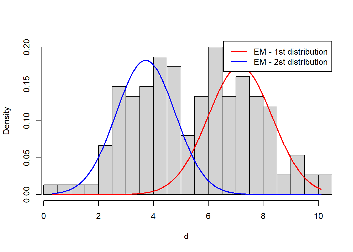

Full source code: https://github.com/mrtkp9993/MyDsProjects/tree/main/EM

References

\(^1\) http://www.columbia.edu/~mh2078/MachineLearningORFE/EM_Algorithm.pdf

\(^2\) https://web.mit.edu/6.435/www/Dempster77.pdf

\(^3\) https://rpubs.com/H_Zhu/246450

Citation

BibTeX citation:

@online{koptur2022,
  author = {Koptur, Murat},
  title = {Under the Hood: {Expectation} {Maximization} {(EM)}},
  date = {2022-10-10},
  url = {https://www.muratkoptur.com/MyDsProjects/EM/Analysis.html},
  langid = {en}
}

For attribution, please cite this work as:

Koptur, Murat. 2022. “Under the Hood: Expectation Maximization (EM).” October 10, 2022. https://www.muratkoptur.com/MyDsProjects/EM/Analysis.html.