How to identify a dynamical system from measurements.
Author
Murat Koptur
Published
September 7, 2022
Introduction
System identification is a way to determine a system’s mathematical description by analyzing the system’s
observed inputs and outputs. Definitely, the dynamics of the mathematical model that produced this signal from
the measured input are hidden inside the output signal; how can this information be extracted? System
identification provides a solution to this problem. Even under ideal conditions, this is difficult because the
model of the system will be unknown, such as whether it is linear or nonlinear, how many terms are in the
model, what type of terms should be in the model, whether the system has a time delay, what type of
nonlinearity describes this system, and so on. Yet, if system is to be useful, these problems must be
resolved. The benefits of system identification are numerous: it is applicable to all systems, it is
frequently fast, and it can be used to track changes in the system\(^1\).
What do we mean with “system”? One can think of “system” as any set of mathematical operations that takes one
or more inputs and produces one or more outputs. Anything that can be related to input and output data is a
system example: electrical systems, mechanical systems, biological systems, financial systems, chemical
systems…\(^3\)
Source: \(^2\)
Systems can be considered of two types, depending on whether they satisfy the principle of superposition:
Linear systems are satisfies the superposition principle: if system is linear, then if input \(X_1\) generates response \(Y_1\) and input
\(X_2\) generates response \(Y_2\), then
input \(X_1 + X_2\) generates response \(Y_1 +
Y_2\).
On the other hand, nonlinear systems does not satisfy the superposition principle. This description is
very vague, but there are so many types of nonlinear systems, it is almost impossible to write down a
description that covers all the classes \(^1\).
Most of real-world dynamical systems are nonlinear. In this article, we will not talk about linearization of
nonlinear systems, as we will focus on the NARMAX method.
Following steps are needed for NARMAX modelling \(^3\):
Collecting data;
Choice of mathematical representation;
Detecting model structure;
Parameter estimation;
Model validation;
Analysis of model.
NARMAX method was introduced in 1981 by Stephen A. Billings, NARMAX models are able to represent the most
different and complex nonlinear systems. NARMAX models can be represented as:
where \(n_y\in \mathbb{N}\), \(n_u \in
\mathbb{N}\) and \(n_e \in \mathbb{N}\) are the maximum lags for the
system output and system input and system noise , respectively; \(x_k \in
\mathbb{R}^{n_x}\) is the system input and \(y_k \in
\mathbb{R}^{n_y}\) is the system output at discrete time \(k \in
\mathbb{N}^n\); \(d\) is the time delay; \(e_k \in \mathbb{R}^{n_e}\) is system uncertainty and noise at discrete time
\(k\), (source: \(^3\)).
To approximate the unknown mapping \(f[\cdot]\), we can use several
nonlinear functions like \(^1\):
Polynomial basis: Polynomial NARMAX model can be written as
where \(\mathbf{x}(k)=[x_1(k),\ldots,x_n(k)]^T\) is the \(k\)th observation vector (\(k=1,2,\ldots,N\)), \(\phi(||\mathbf{x}(k)-\mathbf{x}(i)||\) are some arbitrary nonlinear
functions known as radial basis functions or kernels, and \(W_i\) are the
unknown weights.
where \(F^{(P)}[\mathbf{x}(k)]\) is polynomial model that is used to
model any slow or smooth varying trends, F^{(W)}[(k)] is a wavelet model that is used to model rapid
changes or nonsmooth dynamics, and F^{(Z)}[(k)] is a linear or nonlinear moving average model that models
the noise:
where \(c_0\) is constant and \(F_i[\cdot]\) are individual wavelet sub-models.
Examples
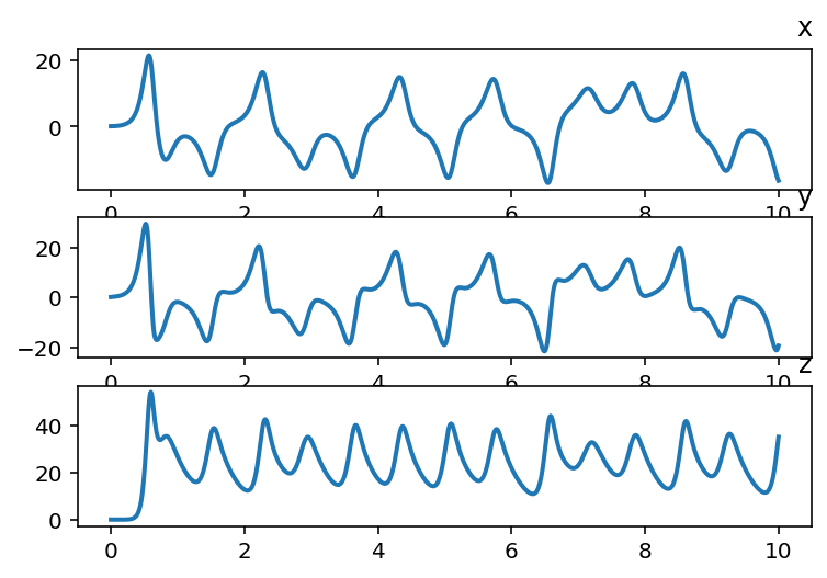
Lorenz system
The Lorenz system is a system of ordinary differential equations defined as:
\[
\begin{align*}
\frac{dx}{dt} &= \sigma(y-x) \\
\frac{dy}{dt} &= x(\rho-z)-y\\
\frac{dz}{dt} &= xy - \beta z
\end{align*}
\] where \(\sigma, \rho, \beta\) are model parameters.
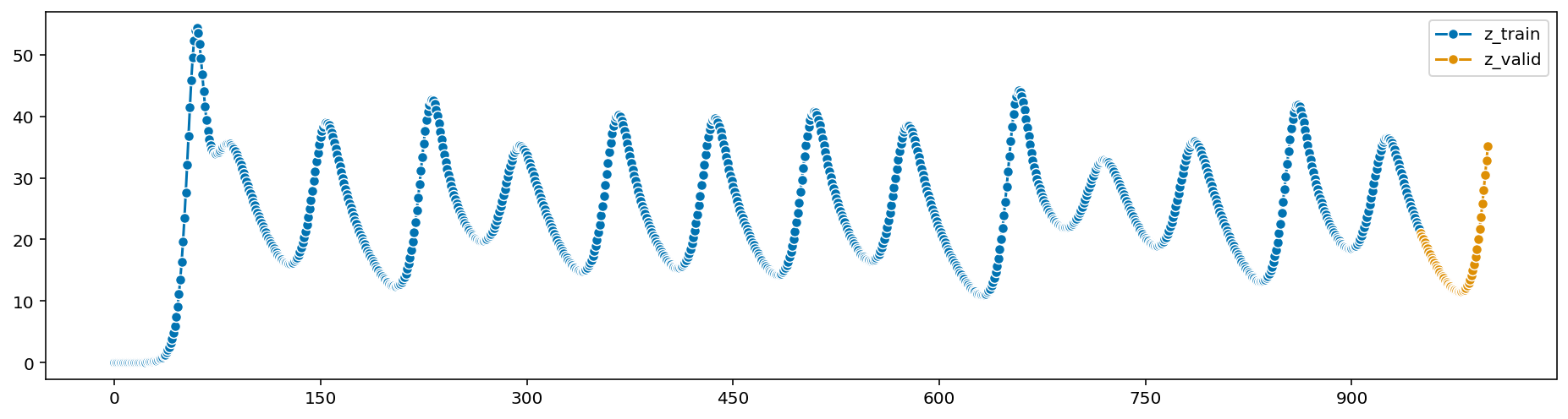
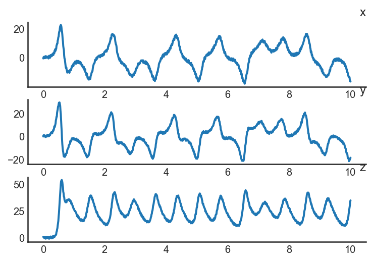
Let’s simulate the data with \(\rho=28, \sigma=10, \beta=8/3\). Here is
the time step \(dt\) is \(0.01\), final
time \(10\), initial values \((x_0,y_0,z_0)\) is \((0.1, 0.1, 0.1)\):
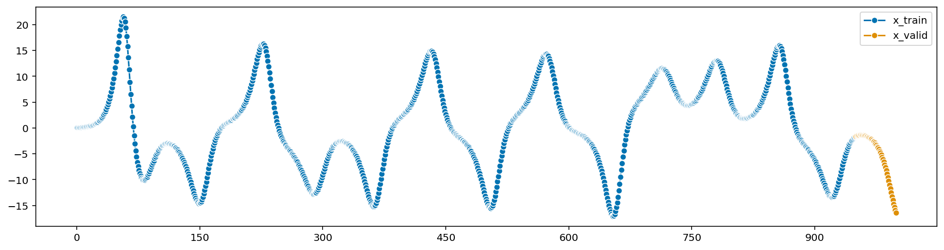
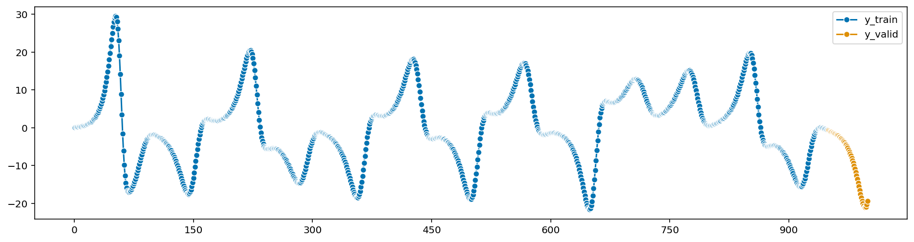
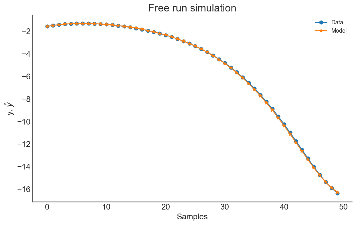
\(y\) and \(z\) components of the Lorenz
model also can be estimated above. Now, let’s add measurement noise to our data and try to estimate it.
Noisy Lorenz System
Now we will assume that we observed the data with independent and identically distributed measurement noise
(we will assume that measurement noise is distributed as uniform on interval [-1, 1]):