X_tr, y_tr = load_from_tsfile_to_dataframe("data/AtrialFibrillation_TRAIN.ts")
X_ts, y_ts = load_from_tsfile_to_dataframe("data/AtrialFibrillation_TEST.ts")Time Series Classification with Random Forests
How to classify time series.
Introduction
First, let’s look the methodology behind the idea.
Suppose that \(N\) training time series examples \(\{e_1,e_2,\ldots,e_N\}\) and the corresponding class labels \(\{y_1,\ldots,y_N\},\quad y_i\in\{1,2,\ldots,C\}\) where \(C\) is the class count, are given. The task is to predict the class labels for test examples. Here, for simplicity, we assume the values of time series are measured at equally-spaced intervals and training and test time series examples are of the same length \(M\) \(^1\).
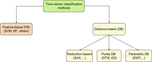
Time series classification methods can be divided into two categories: Instance-based and feature-based. Instance-based methods like nearest-neighbor classifiers with Euclidean distance (NNEuclidean) or dynamic time warping (NNDTW) try to classify test examples based on its similarity to the training examples \(^1\).
Feature-based methods build models on temporal features like \(^3\):
- Singular Value Decomposition (SVD),
- Discrete Fourier Transform (DFT),
- Coefficients of the decomposition into Chebysev Polynominals,
- Discrete Wavelet Transform (DWT),
- Piecewise Linear Approximation,
- ARMA coefficients,
- Symbolic representations like Symbolic Aggregate approXimation (SAX).
Interval Features
Interval features are computed from a time series interval, e.g, “the interval between time 5 and 15”. Let \(K\) be the number of feature types and \(f_K(\cdot),\quad k=1,2,\ldots,K\) be the \(k^{th}\) type. Here the authors of the paper \(^1\) considers three types: \(f_1 = \text{mean}\), \(f_2 = \text{standard deviation}\), and \(f_3=\text{slope}\).
We dont’t go details of the algorithm here, we’ll focus on examples.
Examples
Datasets were downloaded from \(^4\).
Atrial Fibrillation
This is a physionet dataset of two-channel ECG recordings has been created from data used in the Computers in Cardiology Challenge 2004, an open competition with the goal of developing automated methods for predicting spontaneous termination of atrial fibrillation (AF). The raw instances were 5 second segments of atrial fibrillation, containing two ECG signals, each sampled at 128 samples per second. The Multivate data organises these channels such that each is one dimension. The class labels are: n, s and t. class n is described as a non termination artiral fibrilation(that is, it did not terminate for at least one hour after the original recording of the data). class s is described as an atrial fibrilation that self terminates at least one minuet after the recording process. class t is descirbed as terminating immediatly, that is within one second of the recording ending. PhysioNet Reference: Goldberger AL, Amaral LAN, Glass L, Hausdorff JM, Ivanov PCh, Mark RG, Mietus JE, Moody GB, Peng CK, Stanley HE. PhysioBank, PhysioToolkit, and PhysioNet: Components of a New Research Resource for Complex Physiologic Signals. Circulation 101(23):e215-e220 [Circulation Electronic Pages; (Link Here) 2000 (June 13). PMID: 10851218; doi: 10.1161/01.CIR.101.23.e215 Publication: Moody GB. Spontaneous Termination of Atrial Fibrillation: A Challenge from PhysioNet and Computers in Cardiology 2004. Computers in Cardiology 31:101-104 (2004) \(^5\).
Let’s read dataset:
Take a look:
Markdown(tabulate(
  X_tr.head(1),
  headers=X_tr.columns
))| dim_0 | dim_1 | |
|---|---|---|
| 0 | 0 -0.34086 | 0 0.14820 |
| 1 -0.38038 | 1 0.13338 | |
| 2 -0.34580 | 2 0.10868 | |
| 3 -0.36556 | 3 0.09386 | |
| 4 -0.34580 | 4 0.07410 | |
| … | … | |
| 635 -0.04446 | 635 -0.03458 | |
| 636 -0.04940 | 636 -0.05928 | |
| 637 -0.02964 | 637 -0.06916 | |
| 638 -0.01976 | 638 -0.06916 | |
| 639 0.00000 | 639 -0.07410 | |
| Length: 640, dtype: float64 | Length: 640, dtype: float64 |
Markdown(tabulate(
  y_tr,
  headers="Labels"
))
L
n n n n n s s s s s t t t t t
fig, axes = plt.subplots(nrows=2, ncols=1)

X_tr.iloc[0,0].plot(ax=axes[0])
X_tr.iloc[0,1].plot(ax=axes[1])

fig.tight_layout()
fig.subplots_adjust(top=0.88)
fig.suptitle("non termination artiral fibrilation")
plt.show()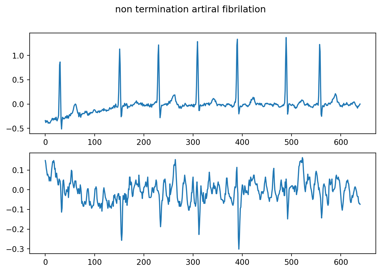
fig, axes = plt.subplots(nrows=2, ncols=1)

X_tr.iloc[6,0].plot(ax=axes[0])
X_tr.iloc[6,1].plot(ax=axes[1])

fig.tight_layout()
fig.subplots_adjust(top=0.88)
fig.suptitle("an atrial fibrilation that self terminates")
plt.show()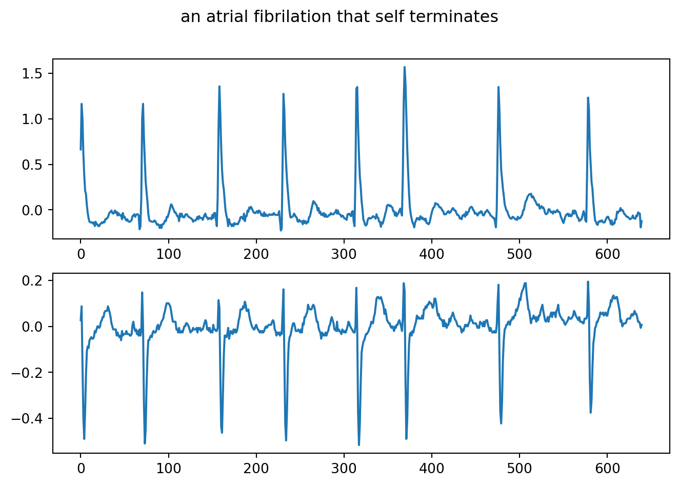
fig, axes = plt.subplots(nrows=2, ncols=1)

X_tr.iloc[12,0].plot(ax=axes[0])
X_tr.iloc[12,1].plot(ax=axes[1])

fig.tight_layout()
fig.subplots_adjust(top=0.88)
fig.suptitle("terminating immediatly")
plt.show()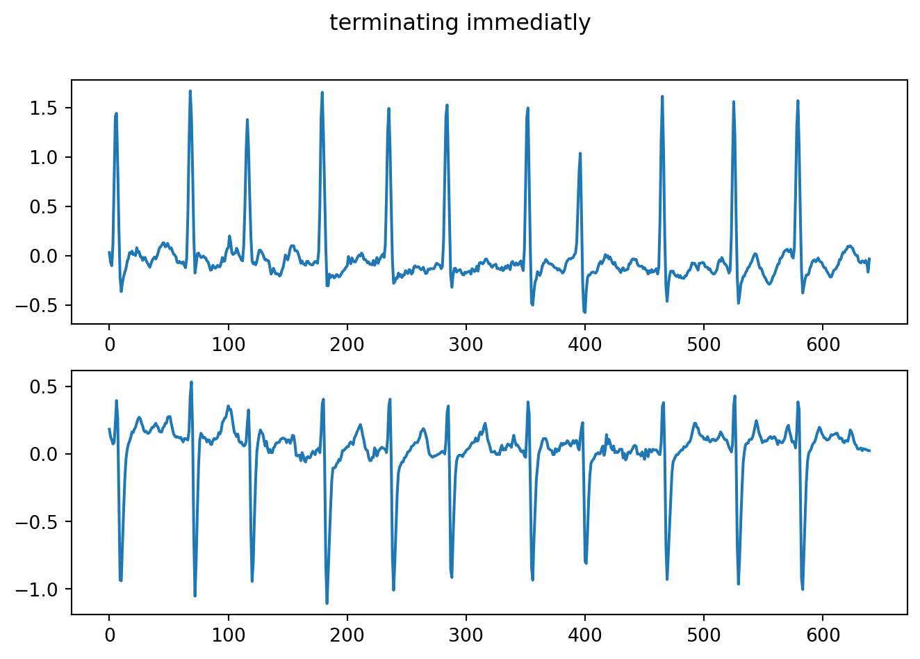
Our data is multivariate. We’ll use ColumnConcatenator which concatenates each dimension and
converts multivariate time series to univariate time series.
cc = ColumnConcatenator()
X_tr = cc.fit_transform(X_tr)
X_ts = cc.fit_transform(X_ts)
Let’s train classifier:
clf = TimeSeriesForestClassifier(min_interval=200, n_estimators=10000, n_jobs=-1, random_state=1234)
clf.fit(X_tr, y_tr)
TimeSeriesForestClassifier(min_interval=200, n_estimators=10000, n_jobs=-1,
random_state=1234)Predict test data and check accuracy:
y_pr = clf.predict(X_ts)
print(classification_report(y_ts, y_pr))
precision recall f1-score support
n 1.00 0.40 0.57 5
s 0.50 0.60 0.55 5
t 0.29 0.40 0.33 5
accuracy 0.47 15
macro avg 0.60 0.47 0.48 15
weighted avg 0.60 0.47 0.48 15
Visualize confusion matrix:
cm = confusion_matrix(y_ts, y_pr, labels=['n', 's', 't'])
ax = sn.heatmap(pd.DataFrame(cm), annot=True, square=True, cbar=False, fmt='g')
plt.xlabel("Predicted")
plt.ylabel("Actual")
ax.invert_yaxis()
plt.show()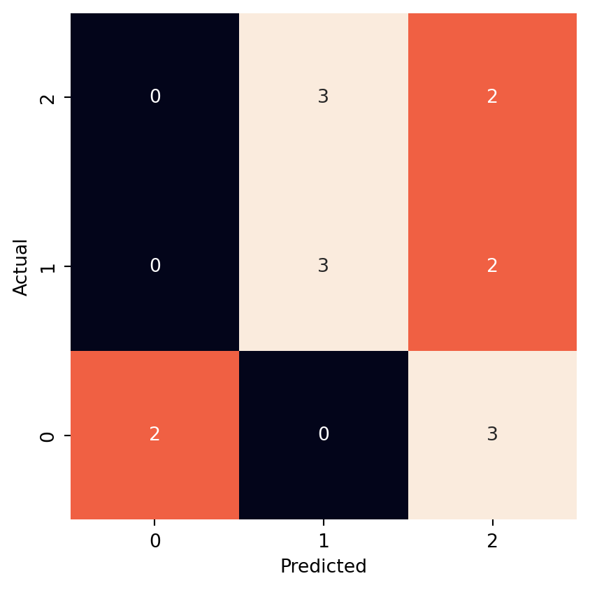
Full source code: https://github.com/mrtkp9993/MyDsProjects/tree/main/TimeSeriesClassification
References
\(^1\) Deng, H., Runger, G., Tuv, E., & Vladimir, M. (2013). A Time Series Forest for Classification and Feature Extraction. arXiv. https://doi.org/10.48550/arXiv.1302.2277
\(^2\) Johann Faouzi and Hicham Janati. pyts: A python package for time series classification. Journal of Machine Learning Research, 21(46):1−6, 2020.
\(^3\) Eruhimov, V., Martyanov, V., Tuv, E. (2007). Constructing High Dimensional Feature Space for Time Series Classification. In: Kok, J.N., Koronacki, J., Lopez de Mantaras, R., Matwin, S., Mladenič, D., Skowron, A. (eds) Knowledge Discovery in Databases: PKDD 2007. PKDD 2007. Lecture Notes in Computer Science(), vol 4702. Springer, Berlin, Heidelberg. https://doi.org/10.1007/978-3-540-74976-9_41
\(^4\) https://www.timeseriesclassification.com/
\(^5\) https://www.timeseriesclassification.com/description.php?Dataset=AtrialFibrillation
No matching items
Citation
BibTeX citation:
@online{koptur2022,
  author = {Koptur, Murat},
  title = {Time {Series} {Classification} with {Random} {Forests}},
  date = {2022-09-17},
  url = {https://muratkoptur.com/MyDsProjects/TimeSeriesClassification/Analysis},
  langid = {en}
}
For attribution, please cite this work as:
Koptur, Murat. 2022. “Time Series Classification with Random
Forests.” September 17, 2022. https://muratkoptur.com/MyDsProjects/TimeSeriesClassification/Analysis.