Don’t Try to Forecast Everything: Predictability of Time Series
We’ll look at a few handy tools that give more information about our time series.
Introduction
Most of time series analyses start with investigating series, autocorrelation and partial autocorrelation plots. Then one estimates different time series models (like ARIMA, GARCH, State-space models) and performs model checks.
But no one asks whether that series is predictable or not.
We’ll look at a few handy tools that give more information about our time series.
Data
We’ll use some example time series:
-
Monthly Airline Passenger Numbers 1949-1960 (AirPassengers) \(^{6}\)
-
Level of Lake Huron 1875-1972 (LakeHuron) \(^{6}\)
-
Simulated time-series data from the Logistic map with chaos \(^{1}\)
Tools
Let’s look the tools.
Lyapunov Exponent
Lyapunov exponent of a dynamical system is a quantity that characterizes the rate of separation of infinitesimally close trajectories. Quantitatively, two trajectories in phase space with initial separation vector \(\delta Z_0\) diverge at a rate given by
\[ |\delta Z(t)|\approx e^{\lambda t}|\delta Z_0| \]
where \(\lambda\) is the Lyapunov exponent. The rate of separation can be different for different orientations of initial separation vector. Thus, there is a spectrum of Lyapunov exponents. It is common to refer to the largest one as the maximal Lyapunov exponent (MLE), because it determines a notion of predictability for a dynamical system \(^{7}\).

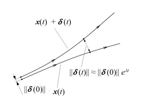
I’ll not go into detail on how to calculate the maximal Lyapunov exponent, we’ll look at practical implications.
A positive MLE is usually taken as an indication that the system is chaotic \(^{7}\).
Hurst Exponent
The Hurst exponent is referred to as the “index of dependence” or “index of long-range dependence”. It quantifies the relative tendency of a time series either to regress strongly to the mean or to cluster in a direction:
-
Trending (Persistent) series: If \(0.5 < H \leq 1\) , then series has long-term positive autocorrelation, so a high value in the series will probably be followed by another high value and the future will also tend to be high;
-
Random walk series: if \(H = 0.5\), then series is a completely uncorrelated series, so it can go either way (up or down);
-
Mean-reverting (Anti-persistent) series: if \(0 \leq H < 0.5\), then series has mean-reversion, so a high value in the series will probably be followed by a low value and vice versa \(^{8}\).
Detrended Fluctuation Analysis
DFA is a method for determining the statistical self-affinity of a signal. It is the generalization of Hurst exponent, it means \(^{8}\):
-
for \(0<\alpha<0.5\), then the series is anti-correlated;
-
for \(\alpha=0.5\), then the series is uncorrelated and corresponds to white noise;
-
for \(0.5<\alpha<1\), then the series is correlated;
-
for \(\alpha\approx1\), then the series corresponds to pink noise;
-
for \(\alpha>1\), then the series is nonstationary and unbounded;
-
for \(\alpha\approx1.5\), then the series corresponds to Brownian noise.
Variance Ratio Test
This test is often used to test the hypothesis that a given time series is a collection of i.i.d. observations or that it follows a martingale difference sequence.
We will use Chow and Denning’s multiple variance ratio test. There are two tests:
- CD1 - Test for i.i.d. series,
- CD2 - Test for uncorrelated series with possible heteroskedasticity.
If test statistics are bigger than critical values, the null hypothesis is rejected which means the series is not a random walk.
Statistics of the series
AirPassengers data
Results:
-
Lyapunov exponent spectrum:
Call:
Lyapunov exponent spectrum

Coefficients:
             Estimate Std. Error   z value      Pr(>|z|)
Exponent 1 -0.8398548  0.2333552 -28.33887 5.739062e-177
Exponent 2 -1.5136329  0.1937088 -61.52719  0.000000e+00
---
Procedure: QR decomposition by bootstrap blocking method
Embedding dimension: 2, Time-delay: 1, No. hidden units: 10
Sample size: 129, Block length: 62, No. blocks: 1000
There are two statistically significant exponent estimates. The largest one is -0.84 which is negative, which means the series is not chaotic.
-
Hurst exponent is 0.8206234; it is bigger than 0.5, so series is trending.
-
DFA is estimated as 1.2988566; it is nonstationary and unbounded.
-
Variance ratio test:
$Holding.Periods
[1]  2  4  5  8 10 27

$CD1
[1] 24.48521

$CD2
[1] 21.22941

$Critical.Values_10_5_1_percent
[1] 2.378000 2.631038 3.142756
Both of test statistics are bigger than critical values, so the series is not a random walk.
LakeHuron data
Results:
-
Lyapunov exponent spectrum:
Call:
Lyapunov exponent spectrum

Coefficients:
             Estimate Std. Error    z value Pr(>|z|)
Exponent 1 -0.2245224 0.03079226  -56.00722        0
Exponent 2 -0.6465142 0.01144893 -433.74968        0
Exponent 3 -0.6696687 0.01006248 -511.18811        0
Exponent 4 -1.6931702 0.02747627 -473.33519        0
---
Procedure: QR decomposition by bootstrap blocking method
Embedding dimension: 4, Time-delay: 1, No. hidden units: 2
Sample size: 94, Block length: 59, No. blocks: 1000
There are four statistically significant exponent estimates. The largest one is -0.22 which is negative, which means the series is not chaotic.
-
Hurst exponent is 0.7364948; it is bigger than 0.5, so series is trending.
-
DFA is estimated as 1.1128455; it is nonstationary and unbounded.
-
Variance ratio test:
$Holding.Periods
[1]  2  4  5  8 10  3

$CD1
[1] 11.45734

$CD2
[1] 9.407748

$Critical.Values_10_5_1_percent
[1] 2.378000 2.631038 3.142756
Both of test statistics are bigger than critical values, so the series is not a random walk.
Simulated time-series data from the Logistic map with chaos
Results:
-
Lyapunov exponent spectrum:
Call:
Lyapunov exponent spectrum

Coefficients:
            Estimate Std. Error   z value Pr(>|z|)
Exponent 1 -1.291195  0.1580609 -63.27662        0
---
Procedure: QR decomposition by bootstrap blocking method
Embedding dimension: 1, Time-delay: 1, No. hidden units: 2
Sample size: 99, Block length: 60, No. blocks: 1000
There is one statistically significant exponent estimate, -1.29 which is negative, which means the series is not chaotic which is a questionable result.
-
Hurst exponent is 0.6255664; it is bigger than 0.5, so series is trending.
-
DFA is estimated as 0.758476; it is correlated.
-
Variance ratio test:
$Holding.Periods
[1]  2  4  5  8 10 10

$CD1
[1] 1.193817

$CD2
[1] 1.295116

$Critical.Values_10_5_1_percent
[1] 2.378000 2.631038 3.142756
Both of test statistics are smaller than critical values, so the series is a random walk.
Full source code: https://github.com/mrtkp9993/MyDsProjects/tree/main/TimeSeriesPredictability
References
\(^1\) DChaos, https://cran.r-project.org/web/packages/DChaos/index.html
\(^2\) statcomp, https://cran.r-project.org/web/packages/statcomp/index.html
\(^3\) pracma, https://cran.r-project.org/web/packages/pracma/index.html
\(^4\) tseriesChaos, https://cran.r-project.org/web/packages/tseriesChaos/index.html
\(^5\) Daniel F. McCaffrey , Stephen Ellner , A. Ronald Gallant & Douglas W. Nychka (1992) Estimating the Lyapunov Exponent of a Chaotic System with Nonparametric Regression, Journal of the American Statistical Association, 87:419, 682-695
\(^6\) boot, https://www.rdocumentation.org/packages/boot/versions/1.3-28/topics/boot.
\(^7\) Contributors to Wikimedia projects. “Lyapunov exponent - Wikipedia.” 7 July 2022, https://en.wikipedia.org/w/index.php?title=Lyapunov_exponent&oldid=1096875011.
\(^8\) Contributors to Wikimedia projects. “Hurst exponent - Wikipedia.” 12 June 2022, https://en.wikipedia.org/w/index.php?title=Hurst_exponent&oldid=1092814465.
\(^9\) DFA, https://cran.r-project.org/package=DFA
\(^{10}\) Contributors to Wikimedia projects. “Detrended fluctuation analysis - Wikipedia.” 19 June 2022, https://en.wikipedia.org/w/index.php?title=Detrended_fluctuation_analysis&oldid=1093832537.
\(^{11}\) nonlinearTseries, https://cran.r-project.org/web/packages/nonlinearTseries/index.html.
No matching items
Citation
BibTeX citation:
@online{koptur2022,
  author = {Koptur, Murat},
  title = {Don’t {Try} to {Forecast} {Everything:} {Predictability} of
    {Time} {Series}},
  date = {2022-09-01},
  url = {https://muratkoptur.com/MyDsProjects/TimeSeriesPredictability/Analysis},
  langid = {en}
}
For attribution, please cite this work as:
Koptur, Murat. 2022. “Don’t Try to Forecast Everything:
Predictability of Time Series.” September 1, 2022. https://muratkoptur.com/MyDsProjects/TimeSeriesPredictability/Analysis.