How to perform uncertainty quantification using polynomial chaos expansion.
Author
Murat Koptur
Published
September 13, 2022
Introduction
Source: \(^4\)
According to \(^2\), uncertainty quantification is defined as
The process of quantifying uncertainties associated with model calculations of true, physical QOIs, with
the goals of accounting for all sources of uncertainty and quantifying the contributions of specific sources
to the overall uncertainty.
and answers the question
How do the various sources of error and uncertainty feed into uncertainty in the model-based prediction of
the quantities of interest?
Types of uncertainties
Aleatoric (statistical) uncertainty refers to the notion of randomness, that is, the variability in the
outcome of an experiment which is due to inherently random effects \(^6\).
Epistemic uncertainty refers to uncertainty caused by a lack of knowledge, i.e., to the epistemic state
of the agent \(^6\).
In real life applications, both kinds of uncertainties are present.
Types of problems
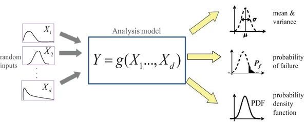
There are two major types of problems in uncertainty quantification: one is the forward propagation of
uncertainty (where the various sources of uncertainty are propagated through the model to predict the overall
uncertainty in the system response) and the other is the inverse assessment of model uncertainty and parameter
uncertainty (where the model parameters are calibrated simultaneously using test data) \(^1\).
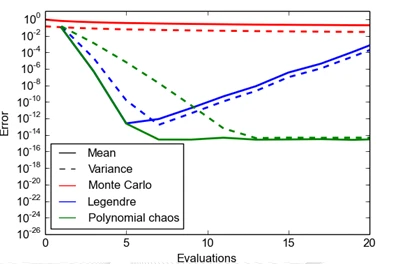
Polynomial chaos is a method for quantifiying uncertainties on forward problems. Its convergence is better
than Monte Carlo methods \(^3\).
Source: \(^3\)
Polynomial Chaos Expansion (PCE)
Consider a problem in space \(x\) and time \(t\) where the aim is to quantify the uncertainty in response \(Y\), computed bu a forward model \(f\), which
depends on uncertain input parameters \(Q\):
\[
Y = f(x,t,Q)
\]
We want to quantify uncertainty in \(Y\), but we know nothing about its
density distribution \(p_Y\). The goal is to either build the density \(p_Y\) or revelant density properties of \(Y\)
using the density \(p_Q\) and the forward model \(f\)\(^5\).
A general polynomial approximation can be defined as
where \(\{c_n\}_{n\in I_N}\) are coefficients and \(\{\Phi_n\}_{n\in I_N}\) are polynomials. If \(\hat{f}\) is a good approximation of \(f\), it
is possible to either infer statistical properties of \(\hat{f}\)
analytically or through numerical computations where \(\hat{f}\) is used as a
surrogate for \(f\)\(^5\).
A polynomial chaos expansion is defined as a polynomial approximation, where the polynomials \(\{\Phi_n\}_{n\in I_N}\) are orthogonal on a custom weighted function space
\(L_Q\):
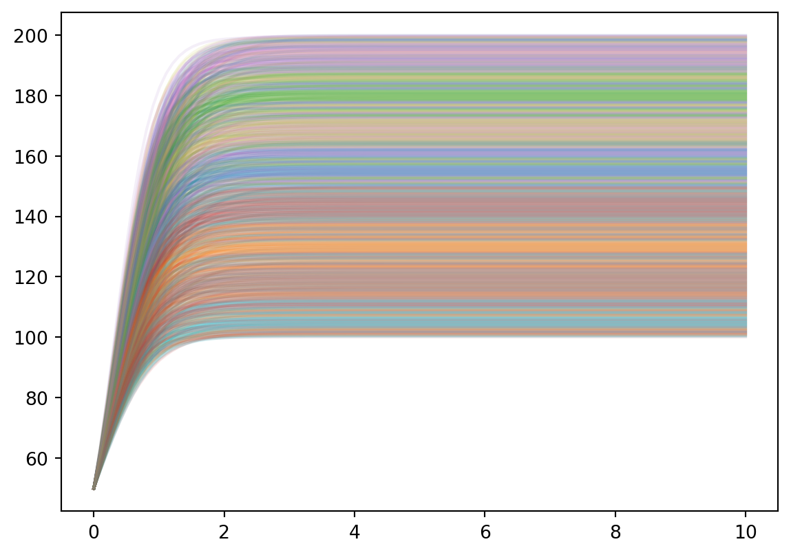
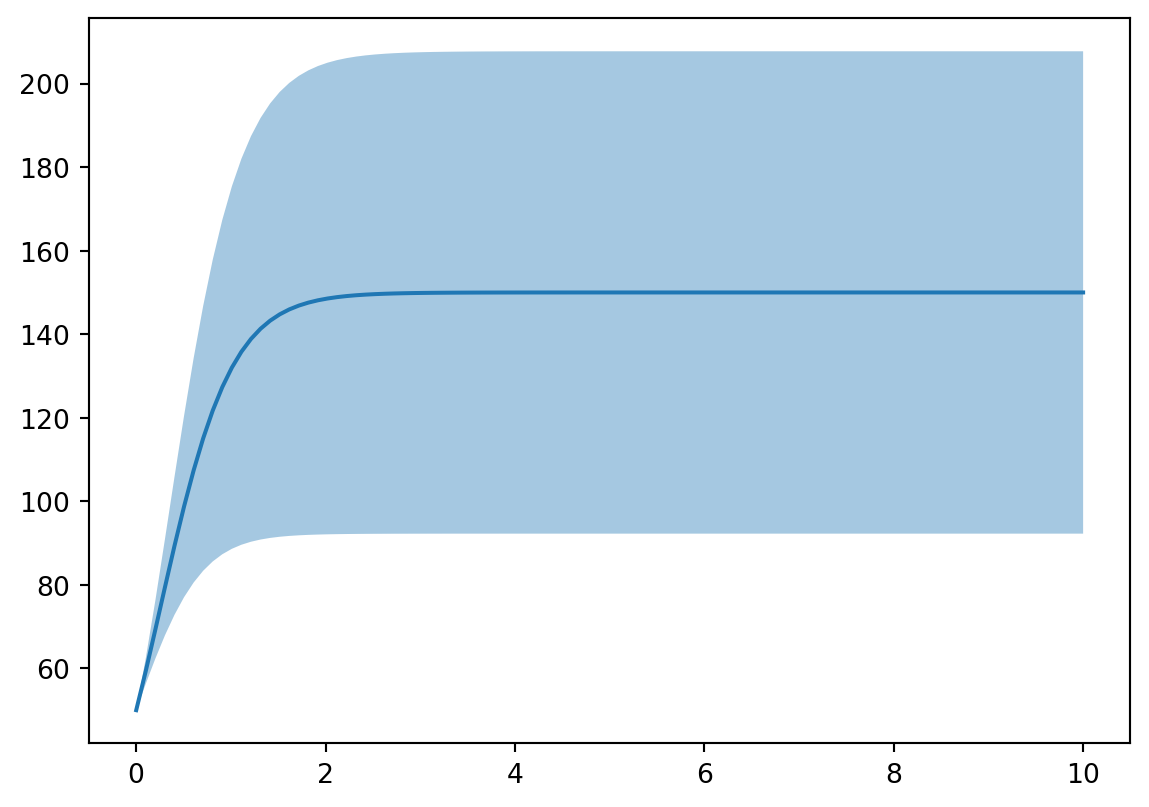
Generate expension, sample the joint distribution, evaluate model at these points and plot:
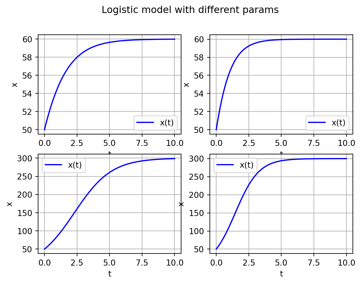
expansion = chaospy.generate_expansion(order=3, dist=joint)# and sample the joint distributionsamples = joint.sample(1000, rule="sobol")# and evulate solver at these samplesevaluations = numpy.array([odeint(logistic_model, x0, t, args=(sample[0], sample[1])) for sample in samples.T])# and plotplt.plot(t, evaluations[:,:,0].T, alpha=0.1)plt.show()
\(^2\) Council, N. R., Engineering and Physical Sciences, D. O.,
Mathematical Sciences and Their Applications, B. O., & Mathematical Foundations of Verification,
Validation, and Uncertainty Quantification, C. O. (2012). Assessing the Reliability of Complex Models. In
Mathematical and Statistical Foundations of Verification, Validation, and Uncertainty Quantification.
\(^5\) Feinberg, J., & Langtangen, H. P. (2015). Chaospy: An open source
tool for designing methods of uncertainty quantification. Journal of Computational Science, 11, 46–57. https://doi.org/10.1016/j.jocs.2015.08.008